As a complement to habitat diversity, the spatial distribution of habitats, e.g. the extent to which habitat types within a landscape alternate (i.e. their spatial heterogeneity) is an important aspect of a varied landscape.
As a measure of spatial heterogeneity, ALL-EMA calculates the Hix index by analysing whether adjacent habitat types are identical or different.
‘Spatial heterogeneity of habitats’ methodology
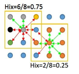
The average Hix index per survey square was calculated according to the method of Fjellstad et al. (2001). Using a ‘moving window’ (yellow-outlined area in the figure on the left), the habitat type of each sampling area was compared with a maximum of eight neighbouring habitat types. Areas not located in the agricultural landscape were not taken into account. If the centre of the habitat type matched the habitat type of the neighbouring square, this relationship was assigned a value of 0. If the neighbouring habitat type differed from that of the centre, the relationship was assigned a value of 1. The average of these relationships was then calculated for each sampling area, with values between 0 (all neighbouring habitat types the same) and 1 (all neighbouring habitat types different) being possible. A high Hix index therefore means that different habitat types were found on a relatively small scale (50-metre grid) in the survey square in question.
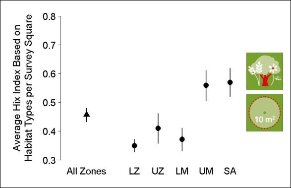
State of spatial heterogeneity of habitats
Contacts
Data reference:
Results